Introduction

The objective of this exploration is to guide you in your first steps of using Thermoptim, by making you discover the main screens and functionalities associated with a simple refrigeration installation model.

You will discover the layout of the screens of the points and the processes, the way in which their parameters can be set and they are calculated, the concepts of useful and purchased energies making it possible to draw up the global energy balances and to determine the Coefficient of Performance COP.

You will plot the cycle in the (h, ln (P)) thermodynamic chart.

If you wish, you can also learn about Thermoptim using the available Diapason sessions, and in particular the Session S07En_init First steps with Thermoptim.

Brief presentation of the refrigerator model

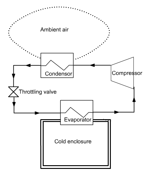
In a vapor compression refrigeration installation, an attempt is made to maintain a cold enclosure at a temperature below ambient

The principle consists in evaporating a refrigerant at low pressure (and therefore low temperature), in an exchanger in contact with the cold enclosure. For this, the evaporation temperature Tevap of the refrigerant must be lower than that of the cold enclosure Tef.

The fluid is then compressed to a pressure such that its condensation temperature Tcond is greater than the ambient temperature Ta.

It is then possible to cool the fluid by heat exchange with the ambient air, until it becomes liquid. The liquid is then expanded without work (we speak of isenthalpic throttling) to low pressure, and directed into the evaporator. The cycle is thus closed.

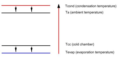This figure illustrates the enthalpy transfers that take place in the facility. Small arrows pointing downwards represent the heat exchange, which, as can be seen, do not infringe the second law of thermodynamics, heat flowing from warmer areas to colder areas. The long upwards arrow represents the enthalpy contribution of the compressor, which can raise the temperature of the fluid (note: the energies put into play are not proportional to the length of arrows).

Setting retained

The compression refrigeration cycle of R134a operates between an evaporation pressure of 1.78 bar and a condenser pressure of 12 bar.

At the outlet of the evaporator, a flow rate $m=1g/s$ of fluid is entirely vaporized, with an superheating of 5 ° C.

It is then compressed to 12 bar following an irreversible adiabatic compression. The actual compression is characterized by an isentropic efficiency, defined as the ratio of the work of the reversible compression to the real work. In this example, its value is assumed to be 0.75

The cooling of the fluid in the condenser by exchange with the outside air involves two stages: desuperheating in the vapor zone followed by condensation.

It is then expanded without work in a capillary, down to the pressure of 1.78 bar.

Main environments of Thermoptim

When you launch the Thermoptim browser, three windows are open:

• the one you are currently reading which contains the html file of the exploration to be carried out
• that of the Thermoptim diagram editor
• that of the Thermoptim simulator

The diagram editor allows one to graphically and qualitatively describe the system studied. It includes a palette presenting the existing components and a work panel where these components are placed and interconnected by vector links.

The simulator allows you to quantify and then calculate the model described in the diagram editor. It includes the lists of the points, processes, nodes and heat exchangers comprising the model.

This document provides more information on these two environments.

Loading a model

Model loading

Click on the following link: Open a file in Thermoptim

Diagram editor window

You can see the diagram of the cycle there, which is almost the same as the one presented above, except that the condenser is represented by two components instead of one.

It has been modeled in this way to clearly show the two thermodynamic changes that take place there: desuperheating of the fluid from 70 ° C to the condensation temperature at 12 bar (46.3 ° C), then condensation at constant temperature.

Press the F3 key, or select the menu item "Special/Display the values".

The diagram then becomes a synoptic view of the installation. On each link between two components, the values ​​of the thermodynamic state of the corresponding point appear (substance name, temperature, pressure, enthalpy) and that of the flow involved (here$1g/s$).

In the title block, the elements of the balance sheet are indicated: useful power, purchased power and efficiency.

If you press the F3 key again, or select the menu item "Special/Display the values", the values ​​are hidden, except those from the title block.

Simulator window

The different elements that make up the model appear in the tables: 5 points and 5 processes, with their main characteristics.

A double-click on one of the lines will display the related screen.

Two important buttons appear in the central part:

• the Balance button allows you to calculate or update the cycle balance
• the Recalculate button allows you to recalculate all the elements of the simulator when one of them has been changed.

We will return to their use later.

Discovery of processes

Screen of a process

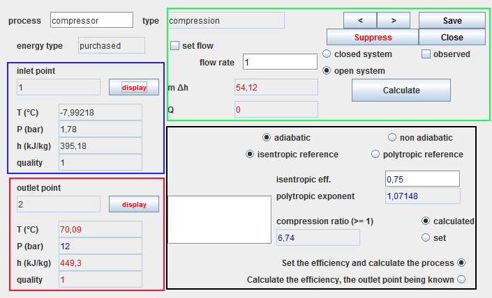
The screen of a process has four main areas, the first three of which are common to all processes:

• the blue zone, in the upper left part, summerizes the state of the upstream point.
• the red zone, in the lower left part, summerizes the state of the downstream point.
• the green zone, in the upper right part, defines the type of system and the flow rate value. It includes the calculation button which determines the power involved $m\Delta h$.
• the black area, in the lower right, contains the specific parameters of the process.
• This document provides more information on these screens.

Sign convention

By convention, we count positively the energies and powers received by a system, and negatively those that it supplies to the outside. This is why the energy or power used in a compressor is counted positively.

Displaying the "compressor" process

How to open the screen of a process?

As an exercise, go to the diagram editor and double-click on the "compressor" process.

If you cannot do it, click this button

Discovery of points

Point screen

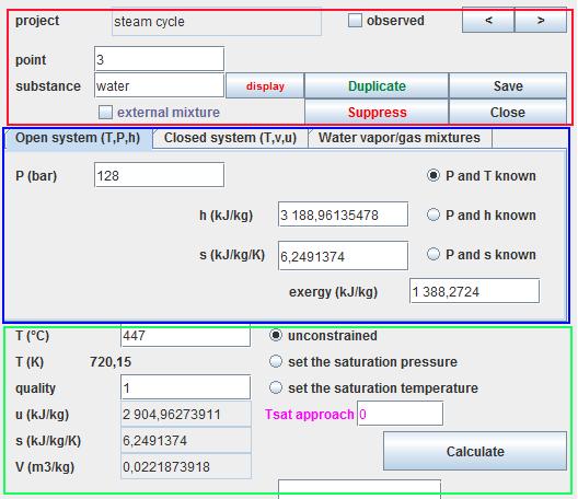
A point screen has three main areas:

• the red zone, in the upper part, where the name of the point and the substance associated with it are defined (here water).
• the blue zone, just below, contains the three tabs which allow you to select the calculation mode (here open systems).
• the green area at the bottom where the point state calculation button is located.

Several settings are possible, especially for vapors, for which it is possible to set the temperature or the saturation pressure.

This document provides more information on these screens.

Showing point "1"

How can you open a point screen?

As an exercise, go to the diagram editor and double-click on the link between processes "refrigeration effect" and "compressor".

If you cannot do it, click this button

The setting of this point has a particularity, at the level of the lower part indicated in green in the image above: the option "set saturation temperature" has been checked, and a value equal to 5 has been entered in the "Tsat approach" field.

This setting is used to tell Thermoptim that the point temperature corresponds to a superheating of 5 ° C compared to the evaporation/condensation temperature at the chosen pressure.

If this pressure is subsequently modified, the point temperature will be automatically recalculated, keeping this superheating value.

Substances in Thermoptim

Displaying a substance

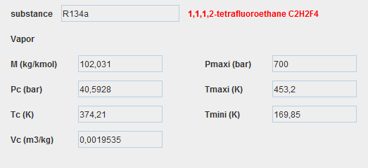
We display a substance in Thermoptim by clicking on the display button located in the upper left part of a point screen.

In our model, the only working fluid is R134a, condensable vapor, the properties screen of which is given below.

Pure gases

Thermoptim includes around twenty pure gases.

The properties of the gases are based on the ideal gas model: the law $Pv=rT$ and a development of the thermal capacity Cp of the gas as a function of the temperature.

The perfect gas corresponds to the particular case where Cp is a constant.

Compound gases

We can define in Thermoptim as many compound gases as desired, obtained by mixing the pure gases available.

Compound gases are divided into two categories:

• protected gases whose composition cannot be modified by a user
• the others, called unprotected.

The reason for this distinction is simply to prevent a modeling error from changing the composition of a known gas, such as that of air or natural gas.

Condensable vapors

About twenty condensable vapors represent fluids in areas close to their liquid-vapor equilibrium curve.

The ideal gas model is therefore insufficient.

External substances

These are substances defined outside of the Thermoptim core, hence their name.

They can either be simple substances, entirely calculated in the external classes of Thermoptim, or else mixtures, whose calculation can be carried out in specific software, coupled with Thermoptim.

Cycle plot in the (h, ln (P)) thermodynamic chart

(h, ln (P)) chart

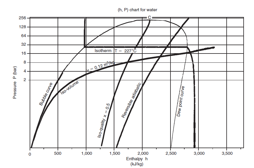
In the (h, ln (P)) chart, the enthalpy is plotted on the abscissa, and the pressure is plotted on the ordinate, most often on a logarithmic scale, so that the area corresponding to the low pressures is more readable.

Its apex corresponds to the critical point C, the left, ascending part, represents the beginning boiling points (bubble curve), and its right, descending part, saturated steam (dew curve).

Between these curves is the domain of the two-phase liquid-vapor equilibrium, and, in the rest of the plane, that of the simple fluid.

This figure, relating to water, recalls the names of the main curves in the chart.

First step: loading the R134a (h, ln (P)) chart

Click this button

Possible modification of the layout of the chart axes

If the layout of the chart axes does not suit you, you can modify it using the lines X Axis and Y Axis of the Chart menu. A layout window is then displayed.

If you click on the "Grid" box, vertical lines for the x-axis and horizontal lines for the y-axis are drawn on the screen, at the main scale of the axis.

If you click on the "Automatic scale" box, Thermoptim will search for a scale covering all the data relating to the selected substance.

The scale is logarithmic if you check the corresponding box, and linear otherwise.

If the "Automatic scale" box is not checked, you can enter the minimum and maximum values ​​you want. The values ​​for the main and secondary scales can either be calculated automatically or entered by you, depending on whether the corresponding "Auto" box is checked or not.

Please note: if the "Automatic scale" box is checked, your values ​​will be replaced by those that Thermoptim will automatically determine.

After making your changes, click "OK" to save your choices, and "Cancel" to return to the previous values.

Second step: loading a pre-defined cycle, the layout of which has been previously refined in order to be more precise

Click this button

Identification of some characteristic points in the chart

Third step: change of chart type: display of the entropy (T, s) chart

To display this type of chart, click this button

If the abscissa or ordinate scale does not suit you, change it using the "Chart/X Axis" and "Chart/Y Axis" menus.

Overall cycle performance, efficiency determination

Energy types of processes

Overall balance

We saw earlier that the cycle balance appears both in the diagram editor and in the simulator screen.

Let's see how it is calculated. In order not to weigh down the discourse, we are talking about energies here, but the reasoning is of course also valid for the capacities.

Identifying the energy types of the model processes

Application: open the various processes of the cycle and find their energy types.

Using the example catalog

Change in model settings

Flow propagation

Application: modification of the model flow

As an exercise, modify the flow rate in this process, for example by entering the value of 2 (g/s) instead of 1.

In order for this value to be taken into account by Thermoptim, you must then click the process "Calculate" button.

To update the complete model, go to the simulator screen and click the "Recalculate" button until the balance stabilizes.

Then go to the diagram editor and press twice the F3 key: the new screen is then displayed. The useful and purchased capacities have doubled, but the efficiency (here the COP) has of course remained the same.

Propagation of pressures

Application: modification of the model high pressure

As an exercise, modify the high pressure in this point, for example by entering the value of 9 (bar) instead of 12.

For this value to be taken into account by Thermoptim, you must click the point "Calculate" button.

Then check the "iso-pressure" option in the "desuperheating" and "condenser" processes.

To update the complete model, go to the simulator screen and click the "Recalculate" button until the balance stabilizes.

Then go to the diagram editor and press twice the F3 key: the new screen is then displayed. The COP has improved since the condensing temperature has dropped.